Resource Modeling Tutorial
Core ABS
ABS is a modeling language which combines functional and imperative
programming styles to develop high-level executable models. Concurrent object
groups execute in parallel and communicate through asynchronous method calls.
To intuitively capture internal computation inside a method, we use a simple
functional language based on user-defined algebraic data types and functions.
Thus, the modeler may abstract from the details of low-level imperative
implementations of data structures, and still maintain an overall
object-oriented design which is close to the target system. At a high level
of abstraction, concurrent object groups typically consist of a single
concurrent object; other objects may be introduced into a group as required to
give some of the algebraic data structures an explicit imperative
representation in the model. In this tutorial, we aim at high-level models
and the groups will consist of single concurrent objects. The functional
sublanguage of ABS consists of a library of algebraic data types such as the
empty type Unit, booleans Bool, integers Int, parametric data types such
as sets Set<A> and maps Map<A> (given a value for the type variable A),
and (parametric) functions over values of these data types. For example, we
can define polymorphic sets using a type variable A and two constructors
EmptySet and Insert, and a function contains which checks whether an
element el is in a set ss recursively by pattern matching over ss:
data Set<A> = EmptySet | Insert(A, Set<A>);
def Bool contains<A>(Set<A> ss, A el) =
  case ss {
    EmptySet      => False ;
    Insert(el, _) => True;
    Insert(_, xs) => contains(xs, el);
  };
Here, the cases p=>exp are evaluated in the listed order, underscore works
as a wild card in the pattern p, and variables in p are bound in the
expression exp. The imperative sublanguage of ABS addresses concurrency,
communication, and synchronization at the concurrent object level in the
system design, and defines interfaces and methods with a Java-like syntax.
ABS objects are active; i.e., their run method, if defined, gets called upon
creation. Statements are standard for sequential composition s1;s2,
assignments x=rhs, and for the skip, if, while, and return
constructs. The statement suspend unconditionally suspends the execution of
the active process of an object by adding this process to the queue, from
which an enabled process is then selected for execution. In await g, the
guard g controls the suspension of the active process and consists of
Boolean conditions b and return tests x? (see below). Just like
functional expressions e, guards g are side-effect free. If g evaluates
to False, the active process is suspended, i.e., added to the queue, and
some other process from the queue may execute. Expressions rhs include the
creation of an object group new C(e), object creation in the group of the
creator new local C(e), method calls o!m(e) and o.m(e), future
dereferencing x.get, and pure expressions e apply functions from the
functional sublanguage to state variables. Communication and synchronization
are decoupled in ABS. Communication is based on asynchronous method calls,
denoted by assignments f=o!m(e) to future variables f. Here, o is an
object expression and e are (data value or object) expressions providing
actual parameter values for the method invocation. (Local calls are written
this!m(e).) After calling f=o!m(e), the future variable f refers to the
return value of the call and the caller may proceed with its execution without
blocking on the method reply. There are two operations on future variables,
which control synchronization in ABS. First, the guard await f? suspends
the active process unless a return to the call associated with f has
arrived, allowing other processes in the object group to execute. Second, the
return value is retrieved by the expression f.get, which blocks all
execution in the object until the return value is available. The statement
sequence x=o!m(e);v=x.get encodes commonly used blocking calls, abbreviated
v=o.m(e) (often referred to as synchronous calls). If the return value of a
call is without interest, the call may occur directly as a statement o!m(e)
with no associated future variable. This corresponds to message passing in
the sense that there is no synchronization associated with the call.
Real-Time ABS
Real-Time ABS is an extension of ABS which captures the timed behavior of ABS models. An ABS model is a model in Real-Time ABS in which execution takes zero time; thus, standard statements in ABS are assumed to execute in zero time. Timing aspects may be added incrementally to an untimed behavioral model. Our approach extends the distributed concurrent object groups in ABS with an integration of both explicit and implicit time.
Deadlines
The object-oriented perspective on timed behavior is captured by deadlines to
method calls. Every method activation in Real-Time ABS has an associated
deadline, which decrements with the passage of time. This deadline can be
accessed inside the method body with the expression deadline(). Deadlines
are soft; i.e., deadline() may become negative but this does not in itself
block the execution of the method. By default the deadline associated with a
method activation is infinite, so in an untimed model deadlines will never be
missed. Other deadlines may be introduced by means of call-site annotations.
Real-Time ABS introduces two new data types into the functional sublanguage of
ABS: Time, which has the constructor Time(r), and Duration, which has
the constructors InfDuration and Duration(r), where r is a value of the
type Rat of rational numbers. The accessor functions timeVal and
durationValue return r for time and duration values Time(r) and
Duration(r), respectively. Let o be an object which implements a method
m. Below, we define a method n which calls m on o and specifies a
deadline for this call, given as an annotation and expressed in terms of its
own deadline. Remark that if its own deadline is InfDuration, then the
deadline to m will also be unlimited. The function scale(d,r) multiplies
a duration d by a rational number r (the definition of scale is
straightforward).
Int n (T x){ [Deadline: scale(deadline(),0.9)] return o.m(x); }Explicit Time
In the explicit time model of Real-Time ABS, the execution time of
computations is modeled using duration statements duration(e1,e2) with best-
and worst-case execution times e1 and e2. These statements are inserted
into the model, and capture execution time which does not depend on the
system’s deployment architecture. Let f be a function defined in the
functional sublanguage of ABS, which recurses through some data structure x
of type T, and let size(x) be a measure of the size of this data structure
x. Consider a method m which takes as input such a value x and returns
the result of applying f to x. Let us assume that the time needed for
this computation depends on the size of x; e.g., the computation time is
between a duration 0.5*size(x) and a duration 4*size(x). An interface I
which provides the method m and a class C which implements I, including the
execution time for m using the explicit time model, are specified as follows:
interface I {
  Int m(T x)
}
class C implements I {
  Int m (T x){
    duration(0.5*size(x), 4*size(x)); return f(x);
  }
}
Implicit Time
In the implicit time model of Real-Time ABS, the execution time is not
specified explicitly in terms of durations, but rather observed on the
executing model. This is done by comparing clock values from a global clock,
which can be read by an expression now() of type Time. We specify an
interface J with a method p which, given a value of type T, returns a
value of type Duration, and implement p in a class D such that p
measures the time needed to call the method m above, as follows:
interface J {
  Duration p (T x)
}
class D implements J (I o) {
  Duration p (T x){
    Time start; Int y;
    start = now();  y=o.m(x);
    return timeDifference(now(),start);
  }
}
Observe that by using the implicit time model, no assumptions about execution times are specified in the model above. The execution time depends on how quickly the method call is effectuated by the called object. The execution time is simply measured during execution by comparing the time before and after making the call. As a consequence, the time needed to execute a statement with the implicit time model depends on the capacity of the chosen deployment architecture and on synchronization with (slower) objects.
Modeling Deployment Architectures in ABS
Deployment Components
A deployment component in Real-Time ABS captures the execution capacity
associated with a number of concurrent object groups. Deployment components
are first-class citizens in Real-Time ABS, and provide a given amount of
resources which are shared by their allocated objects. Deployment components
may be dynamically created depending on the control flow of the ABS model or
statically created in the main block of the model. We assume a deployment
component environment with unlimited resources, to which the root object of a
model is allocated. When objects are created, they are by default allocated
to the same deployment component as their creator, but they may also be
allocated to a different component. Thus, a model without explicit deployment
components runs in environment, which does not impose any restrictions on the
execution capacity of the model. A model may be extended with other
deployment components with different processing capacities. Given the
interfaces I and J and classes C and D defined in above, we can for
example specify a deployment architecture in which two C objects are
deployed on different deployment components server1 and server2, and
interact with the D objects deployed on a deployment component
clientServer. Deployment components in Real-Time ABS have the type DC and
are instances of the class DeploymentComponent. This class takes as
parameters a name, given as a string, and a set of restrictions on resources.
The name is mainly used for monitoring purposes. Here we focus on resources
reflecting the components’ processing capacity, which are specified by the
constructor CPUCapacity(r), where r represents the amount of abstract
processing resources available between observable points in time. Below, we
create three deployment components Server1, Server2, and ClientServer,
with the processing capacities 6, 3, and unlimited (i.e., ClientServer has
no resource restrictions). The local variables server1, server2, and
clientServer refer to these three deployment components, respectively.
Objects are explicitly allocated to the servers by annotations; below,
object1 is allocated to Server1, etc.
{ // This main block initializes a static deployment architecture:
  DC server1 = new DeploymentComponent("Server1",set[CPUCapacity(6)]);
  DC server2 = new DeploymentComponent("Server2",set[CPUCapacity(3)]);
  DC clientServer = new DeploymentComponent("ClientServer", EmptySet);
  [DC: server1] I object1 = new cog C;
  [DC: server2] I object2 = new cog C;
  [DC: clientServer] J client1monitor = new cog D(object1);
  [DC: clientServer] J client2monitor = new cog D(object2);
}
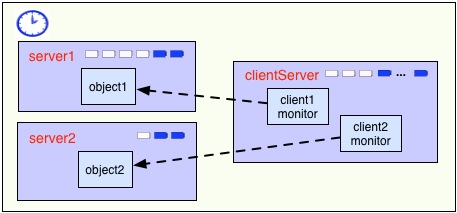
The figure depicts this deployment architecture and the artefacts introduced
into the modeling language. Since all objects are allocated to a deployment
component (which is environment unless overridden by an annotation), we let
the expression thisDC() evaluate to the deployment component of an object.
For convenience, a call to the method total("CPU") of a deployment component
returns its total amount of allocated CPU resources.
Resource Costs
The available resource capacity of a deployment component determines how much computation may occur in the objects allocated to that component. Objects allocated to the component compete for the shared resources in order to execute, and they may execute until the component runs out of resources or they are otherwise blocked. For the case of CPU resources, the resources of the component define its processing capacity between observable (discrete) points in time, after which the resources are renewed.
Cost models
The cost of executing statements in the ABS model is determined by a default
value which is set as a compiler option (e.g., defaultcost=10). However,
the default cost does not discriminate between statements and we may want to
introduce a more refined cost model. For example, if e is a complex
expression, then the statement x=e should have a significantly higher cost
than skip in a realistic model. For this reason, more fine-grained costs
can be inserted into Real-Time ABS models by means of annotations. For
example, let us assume that the cost of computing the function f(x) defined
in the section on Real-Time ABS may be given as a function g which depends
on the size of the input value x. In the context of deployment components,
we may redefine the implementation of interface I above to be
resource-sensitive instead of having a predefined duration as in the explicit
time model. The resulting class C2 can be defined as follows:
class C2 implements I {
  Int m (T x){ [Cost: g(size(x))] return f(x);
  }
}
It is the responsibility of the modeler to specify an appropriate cost model.
A behavioral model with default costs may be gradually refined to provide more
realistic resource-sensitive behavior. For the computation of the cost
functions such as g in our example above, the modeler may be assisted by the
COSTABS tool, which computes a worst-case approximation of the cost for f in
terms of the input value x based on static analysis techniques, when given
the ABS definition of the expression f. However, the modeler may also want to
capture resource consumption at a more abstract level during the early stages
of system design, for example to make resource limitations explicit before a
further refinement of a behavioral model. Therefore, cost annotations may be
used by the modeler to abstractly represent the cost of some computation which
remains to be fully specified. For example, the class C3 below represents a
draft version of our method m in which the worst-case cost of the computation
is specified although the function f has yet to be introduced:
class C3 implements I {
  Int m (T x){ [Cost: size(x)*size(x)] return 0;
  }
}